How to build a clustering model: A comprehensive guide

You already understand at a high level what clustering is and why marketers should care. Let’s get into what it takes to build a working clustering model.

This post assumes you have access to machine learning modeling resources. If you don’t, feel free to sign up for Analyzr, our no-code modeling tool. We illustrate the clustering modeling steps below with Analyzr examples, but you can follow the same steps with any other modeling tool, such as a Jupyter notebook or another machine learning platform.

The five steps to building a clustering model

Building a clustering model involves five steps. We will cover the process end to end. If you are interested primarily in technical topics, such as algorithm selection, go straight to Step 4.

• STEP 1: Create a dataset. Compile an aggregated dataset ready to use by your model.
• STEP 2: Create a model. Create a clustering model instance in your platform of choice.
• STEP 3: Explore your dataset. Explore and validate the dataset prior to using it in your model.
• STEP 4: Configure and train your model. Select relevant variables and choose an algorithm so you can start training your clustering model.
• STEP 5: Predict using your model. Apply your clustering model to a new dataset to make predictions.

While some analysts will complete Step 3 (data exploration) before Step 2 (model creation), we go through this specific order here, as it is more efficient to do so when working from a single tool. In practice, you may find it helpful to go through a fair amount of data exploration on your own prior to using any modeling tool.

STEP 1: Create a dataset

Take the time to assemble a dataset combining all the relevant attributes you know about each prospect or customer, e.g., in the case of customer retention analytics whether a customer has canceled service and all related demographic and usage data. By way of illustration, we will use the Telco Customer Churn dataset, a publicly available dataset. While this dataset is ready to use for modeling, in practice you will spend a fair amount of time compiling your own dataset.

Best practices for compiling datasets will be the subject of a future post. You will need to use a combination of database platforms such as Snowflake, Amazon Redshift, Azure Synapse, or Google Big Query, and your business intelligence tool of choice such as Tableau, PowerBI, or Looker.

Once you’ve assembled your dataset, if you are using a Jupyter notebook, this is the part in your notebook where you would add a line of code to load your dataset. If you are using Analyzr, you will simply go the Datasets page and create a new dataset using the CSV file that contains your data. In our example, we are using the CVS file that we downloaded of the Telco Customer Churn dataset. Make sure you convert the churn outcome to a Boolean value (1 or 0) prior to uploading.

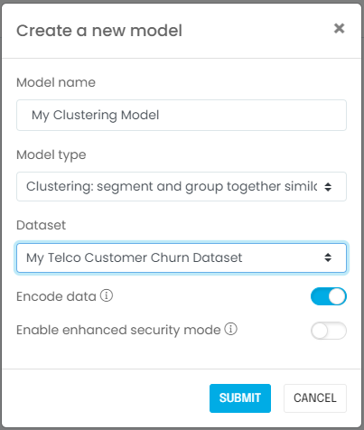
STEP 2: Create a model

Next, you will create a model associated with your dataset. If you are using a Jupyter notebook, this is when you import the relevant machine learning libraries such as scikit-learn, Vaex, or Dask. If you are using Analyzr, you simply go to the Models page and create a new model:

STEP 3: Explore your dataset

It is important to validate that you have the right dataset, and establish some observations or hypotheses about the population you are trying to analyze. You should ask yourself the following questions:

• Is the sample size adequate? In most cases you will need at least a few thousand rows to produce meaningful results. In our example using the telco customer churn dataset, there are more than 7,000 records, so we should be fine.
  
• Did you include known major business drivers in the dataset? In our current example, we know from prior experience that number and type of services affect churn rates, and we included these in the dataset.
  
• Are you aware of meaningful changes over time that would affect the learning process? In other words, are you confident we can infer today’s behavior using yesterday’s data? In our example, the answer is “yes,” because we do not expect customer behavior to change.
  
• Last but not least, did you ingest the correct dataset properly? Does it look right in terms of number of rows, values appearing, etc.? It is fairly common for data to be corrupted if it is not handled using a production-grade process.
  

Congratulations! Now that you’ve answered these questions, you are ready to configure your propensity model.

STEP 4: Configure and train your model

In this step, we will start by selecting variables and an algorithm. We will then train our model to interpret the results. You will need to identify and select two types of variables:

• Independent variables: These are your model inputs, sometimes called drivers or attributes, which will determine business outcomes for your customers. These can be of any type (i.e., numerical, categorical, Boolean). You don’t have to know beforehand which variable is a relevant input, that’s what the training stage will determine. You only need to pick any variable that you think might be relevant and needs to be included.
• An index variable: While this is technically not needed in theory, in practice it’s always an excellent idea to designate a record index that will positively and uniquely identify each record you are processing. It usually is the account ID or customer ID. This will allow you to audit your results and join them back to your original dataset.

Next, you will need to consider the following data manipulation issues. If you are using a Jupyter notebook, you would select the relevant columns of a data frame.

• What is the fill rate for the variables you selected? If you combine too many variables with low fill rates (i.e., a lot of missing values), the resulting dataset will have very few complete rows unless you fill in missing variables (see below).
  
• If you have missing values, what in-fill strategy should you consider? The most common strategies are (i) exclude empty values, (ii) replace empty values with zeros, (iii) replace empty values with the median of the dataset if the variable is numerical, or (iv) replace empty values with the “Unknown” label if the variable is categorical. Using option (ii) or option (iii) usually requires considering what the variable actually represents. For instance, if the variable represents the number of times a customer contacted support, it would be reasonable to assume an empty value means no contact took place and replace empty values with zeros. If the variable represents the length of time a customer has been with the company, using a median might be more appropriate. You will need to use your domain knowledge for this.
  
• Are you including variables with poor data quality that will introduce meaningful biases and artifacts in the clustering results? For instance if too many records are missing in a major variable and get included with a default value, this set of records will likely be identified as its own cluster even though this grouping has no relation to actual customer behavior; it is simply a reflection of data artifacts.
  
• Likewise, do you have outliers in your dataset? Do these outliers reflect reality or are they caused by data quality issues? If it is the latter you will need to remove outliers; if not they will bias your clustering results.
  

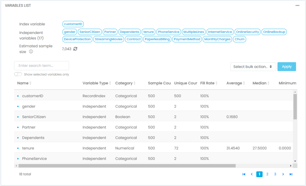
These data manipulations and validation steps are typically tedious with Jupyter notebooks but can be done straightforwardly with several tools, including Analyzr. In our example using the telco customer churn dataset, you will end up with 1 index variable and 17 independent variables selected:

Once you’ve selected and pre-processed your variables, you will need to select an algorithm. The most common choices are:

• PCA K-Means. When in doubt use this general purpose algorithm. Its incremental implementation will scale reasonably well. The PCA step will generally identify natural groupings in the data driven by the same external process. It can be implemented in different ways. With the simple, most straightforward implementation you get to pick the number of clusters you need. With the MLE (Maximum Likelihood Estimator) method the number of clusters can be automatically determined by the number of PCA components.
• K-Means. The traditional and perhaps best known clustering algorithm. It will scale well but usually does not identify more nuanced groupings in the data. Use it only for straightforward clustering cases when you expect clearly separated, convex clusters.
• BIRCH. The BIRCH (balanced iterative reducing and clustering using hierarchies) algorithm is designed to handle larger datasets and as well as noisy data, outliers, etc. In practice it tends to be fairly sensitive. You may want to try it and fall back on the PCA K-Means simple method if this fails to produce meaningful clusters.
• DBSCAN. The DBSCAN (density-based spatial clustering of applications with noise) algorithm was designed with the same objectives as BIRCH, i.e. handle large datasets with noise and outliers. It handles non-convex / uneven clusters more effectively than most. It will also automatically determine the number of clusters. In practice it can be fairly sensitive, esp. with unevenly distributed datasets.
• Gaussian Mixture. The Gaussian Mixture algorithm assumes the dataset to be the superposition of independent, convex clusters. It works reasonably fast on smaller datasets but does not scale well. Use it as validation of the clusters you might have generated with another algorithm.
• Agglomerative Hierarchical. The Agglomerative Hierarchical Clustering algorithm is designed to work well on large datasets with large numbers of clusters. In practice this hierarchical approach may be impacted by the order of the data, and does not always scale well. Use it as validation of the clusters you might have generated with another algorithm such as PCA K-Means.
• Mean Shift. The Mean Shift clustering algorithm is designed to work on smaller datasets with complex, non-convex clusters with outliers. It will automatically determine the number of clusters. However, it does not scale well with larger datasets.
• OPTICS. The OPTICS (ordering points to identify the clustering structure) algorithm is similar to BIRCH and DBSCAN but is specifically designed to handle unevenly distributed datasets. This algorithm in practice can be as sensitive as its two predecessors. Try it first then fall back on the PCA K-Means simple method if needed.
• Spectral Clustering. The Spectral Clustering method is designed to handle a wide variety of cluster shapes but does not scale well. Use it to validate clustering results on small datasets. Fall back on the PCA K-Means simple method if needed.

In our example using the telco customer churn dataset, we will select PCA K-Means (simple method). Note that unless you have a specific reason to pick a different algorithm, you will generally do well using PCA K-Means; it is a general purpose algorithm that does well with most tabular data used by business analysts.

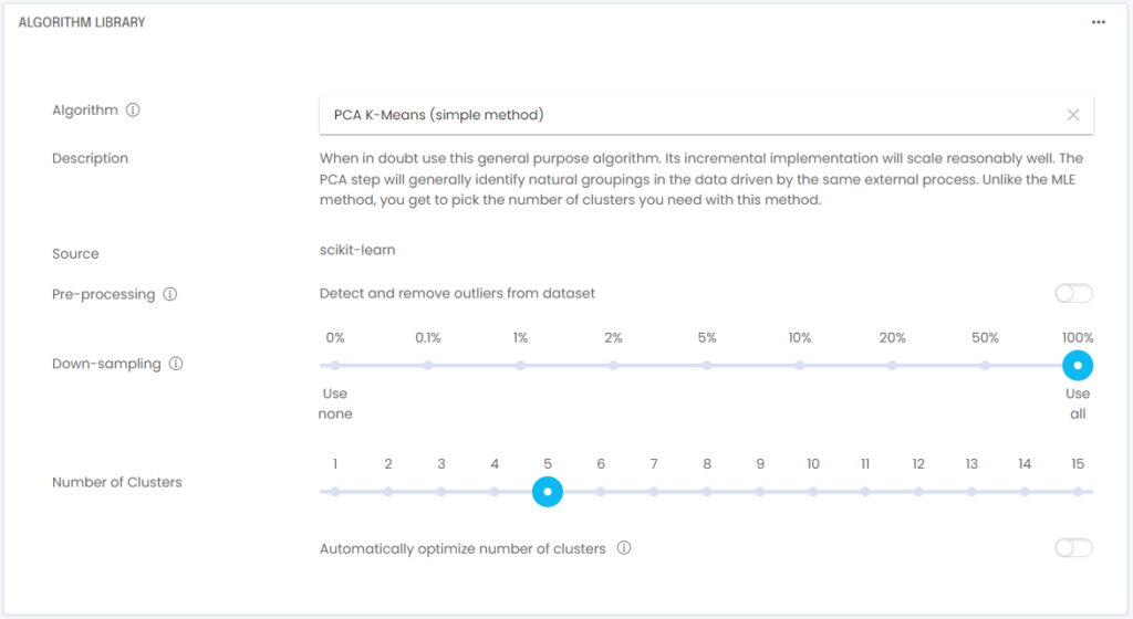
Since there are no outliers in our dataset we will not turn on outlier removal; if you have a different dataset you should consider whether outlier removal is appropriate.

Another practical tip is to down-sample your dataset while you are still tweaking your model. In most cases, testing training on runs of a few thousand rows will be a faster and more efficient way to troubleshoot your model. Once you feel your model is configured properly, you can do a full training run on 100% of the training data. In our example using the telco customer churn dataset, the sample size is small enough that we don’t need to down-sample.

With your variables and algorithm selected, you are now ready to train your model. In a Jupyter notebook, you typically train by invoking the fit() function. In a no-code tool such as Analyzr, you simply go to the Train Model screen and click start. Once training is complete, you will get a set of clusters:

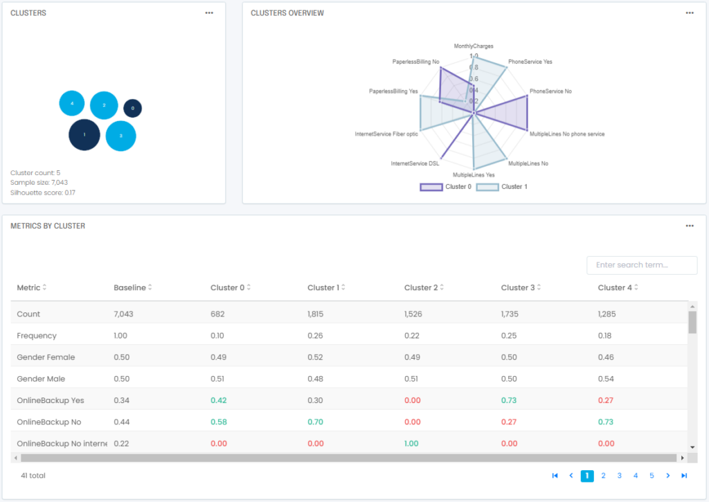
It is important to inspect each cluster and look at sample size as well as averages for key attributes to understand what makes this particular cluster different from the rest of the population. A tool like Analyzr makes it easy to inspect and compare each cluster as shown above.

Unlike classification and regression, clustering does not come with a lot of error metrics. The Silhouette score is a common metric used to quantify the cohesion and separation of clusters produced by a clustering algorithm. It ranges between -1 and +1. With typical tabular data used for business analysis you will want a positive Silhouette score. Other less common metrics include the Davies-Bouldin index and the Dunn index.

While a naïve approach to clustering would be to simply pick a number of clusters that maximizes the Silhouette score, in practice it can lead you astray as the supposedly optimal number may be biased by a number of data artifacts, it may also not align with meaningful business context not included in the data. As a practitioner you are better off manually selecting a number of clusters and inspecting the results yourself, interpreting them using your domain experience. When in doubt, n = 5 is a good place to start.

Another common issue with clustering is the lack of transparency in how the clusters were derived. To better understand what variables and attributes contributed to generating your clusters, it is a good idea to run a classifier on the clustering results and look at the classifier’s feature importance chart (labeled metrics rankings below) to understand how the clusters were formed. If you are using a Jupyter notebook you will need to run a classifier on your clustering results using cluster ID as the outcome you are trying to predict. See for instance this guide on how to do so. With Analyzr the platform will automatically run this step for you when presenting clustering results:

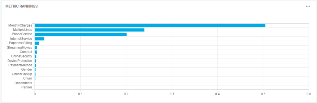
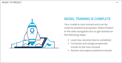
Note that in our example with the telco customer churn example, the monthly charges amount, the number of lines per customers, and whether customers use a phone line in addition to the Internet were key in producing the clusters we saw above. If you’ve made it to this point, congratulations! Your model is now trained.

STEP 5: Predict using your model

At this point you may be wondering: wait, clustering is an unsupervised technique, why do we have a predict step in addition to a training step?

In theory you are correct, we should be able to cluster a dataset and be done. In practice, clustering is used to established a segmentation scheme on a reference dataset of say prospects or customers. Once new prospects or new customers are added to your database, you usually don’t want to or dont need to re-run the clustering algorithm. This would change your segmentation scheme even if only a little bit, and this would have a downstream impact on other sales and marketing activities that depend on your segmentation.

You are better off simply assigning the new records to the closest existing cluster. This way new records will be consistently tagged with a proper cluster ID using the existing segmentation scheme.

How can we help?

Now you’re familiar with the basic steps involved in building a clustering model. Feel free to check us out at https://analyzr.ai or contact us below!